PID controllers are most commonly used to influence certain measured variables. As clever 3-in-1 controllers, they prove themselves every day in numerous industrial systems and control very precisely to the setpoint. Here you can find out the most important facts and figures about PID control.
A digital PID controller can be universally programmed and parameterized by an integrated microprocessor. It operates proportionally, integrating and differentiating (PID), whereby the intensity of the individual components is adapted to the controlled system. This is done by dimensioning the control parameters
The principle of a PID controller is relatively simple to explain. No matter whether the controller is a PID temperature controller or a PID humidity controller, the controller always attempts to adjust a specific control variable to the setpoint value based on the actual value. In this case, the P component amplifies the control deviation, the I component increases its output level in case of existing control deviation, and the D component counteracts the movement of the actual value. Components that are not required for control can be deactivated. Depending on the application, they are then operated as PI controllers, P controllers, PD controllers, or I controllers.
For most applications, the PID structure has the best control behavior. For example, PID compact controllers are very common in the field of temperature control, they also allow direct connection of resistance thermometers and thermocouples. Some controlled variables require disabling of certain components, including speed and flow, among others.
The P component reacts very quickly and amplifies the control difference; its permanent control deviation has a negative effect. The responsible control parameter is the proportional band Xp. With smaller dimensioned Xp the controller becomes faster and the control deviation smaller. However, the overall system tends to oscillate more and more.
The I component eliminates the control deviation. If the reset time Tn is set smaller, the controller builds up its output level faster and also counteracts the control deviation faster. However, if the setting is too small, oscillatory behavior will also occur.
The D component counteracts the movement of the actual value. For a controller for heating, this means that the proportion is reduced when the actual value increases and increased when the actual value decreases. The described behavior has a damping effect. The responsible parameter is the derivative time Tv. The greater Tv is set, the greater is the described effect.
The behavior of controlled systems always depends on the operating point. Therefore, before optimization, the plant must be set to an operating state for which favorable control parameters are expected later. For example, a kiln is loaded before optimization, and an acceptance must be generated for an instantaneous water heater. If a setpoint has to be specified during optimization, it will be in the later operating range.
If comparable plants/control loops exist, the control parameters used there can be used on a trial basis. If this approach does not lead to the goal, one of the following optimization methods can be used.
Vibration method according to Ziegler and Nichols
This method is used for relatively fast controlled systems. For preparation, the P structure is parameterized and a relatively large XP is set. A setpoint in the later working range is defined in the following figure.
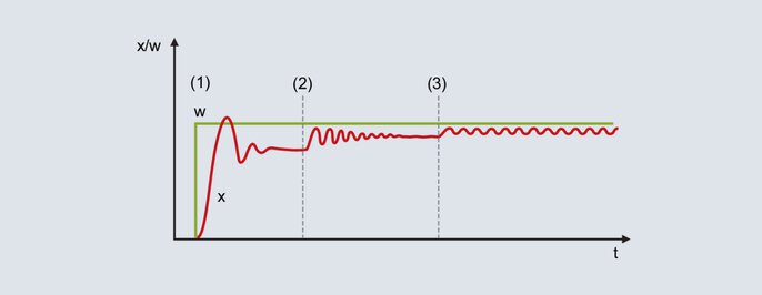
Fig. 52: Setpoint and actual value curve when using the oscillation method
With the relatively large proportional band set, the actual value runs to the final value with a low tendency to oscillation [Figure 52 (1)]. Due to the non-existent I-structure, a permanent control deviation is present.
The XP is reduced (Figure 52 [2]): The actual value increases and runs to the final value with a greater tendency to oscillation. The proportional band may be reduced several times until the actual value oscillates permanently (Figure 52 [3]). The proportional band required for this behavior is called XPk (critical Xp) and must be determined as precisely as possible (do not reduce Xp in too large steps).

Critical period
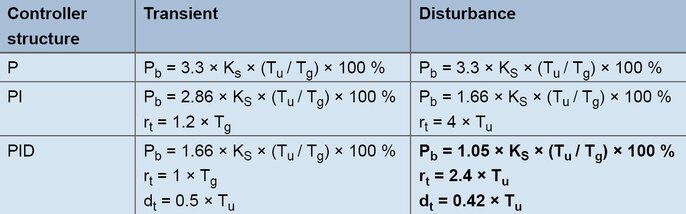
From the continuous oscillation of the actual value in the upper figure, the critical period TK is used to determine the second parameter for the process. The critical period TK (in seconds) results for example from the time interval between 2 minimum values. XPk and TK are inserted into the following table for the desired controller structure:
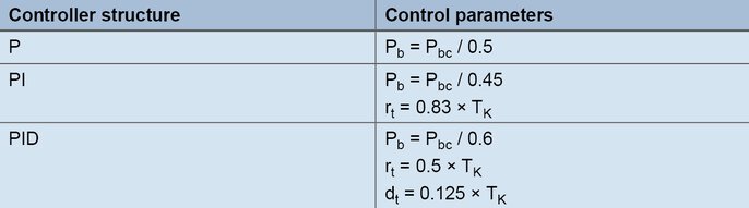
Formulas for setting according to the oscillation method
Procedure according to the distance step response of Chien, Hrones and Reswic
With this method, the control parameters are determined in a relatively time-saving manner even for sluggish controlled systems. The method is used for controlled systems of 2nd order and higher and offers the special feature of differentiating between the formulas for the command and disturbance response. For the rule of thumb formulas, the transfer coefficient of the controlled system, the delay time and the compensation time are determined from the step response.
Formulas for creation according to the line step response
Example:
A digital controller with PID structure is to be used for a laboratory furnace. The aim is to achieve good disturbance behavior, typical setpoints are 200 °C. In manual mode, the output level is increased in steps until the actual value is slightly below the later setpoint (the compensation processes must be waited for in each case). For example, a temperature of 180 °C is reached with an output level of 60 %. Starting from 60 %, the output level is increased in steps to 80 % and the actual value is recorded.
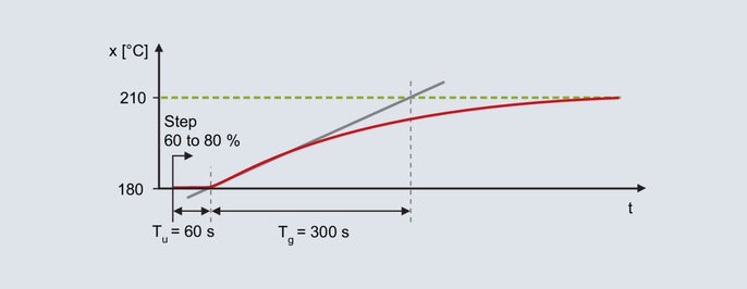
Step response of the laboratory furnace
The step response is determined with the aid of the turn tangent: Delay time Tu = 60 s, compensation time Tg = 300 s. The transmission coefficient of the controlled system results from the change in the actual value divided by the output step.

Equation 22
Using the rules of thumb, the following parameters for the interference behavior result:

Equation 23

Equation 24

Equation 25
The output step must be performed in the range of the subsequent operating point. The step height must still be selected so large that the process value curve can be evaluated. After specifying the output step, the final value of the actual value is waited for; a time-saving alternative is the procedure according to the rate of rise.
Procedure according to the rate of rise
With regard to the step response, the procedure is the same as for the distance step response procedure. Before the step change, an output level is specified with which the actual value is slightly below the setpoint value used later.
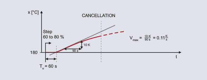
Actual value curve for the method according to slew rate
The step setting is again made for the laboratory furnace already mentioned; the subsequent operating point is also 200 °C. By specifying a degree of operation of 60 % in manual mode, an actual value of 180 °C is obtained. The output level is increased in steps to 80 %.
After presetting the step, the actual value increases after some time. Recording continues until the actual value reaches its maximum slope. Also with this method, the turning tangent is drawn in and the delay time is determined. The second parameter is the maximum rate of rise, this corresponds to the slope of the turn tangent. The maximum rate of ascent is determined by a gradient triangle at the turn tangent:

Equation 26
Die ermittelten Werte Vmax (0,11 K/s) und Tu (60 s) werden in folgende Formeln eingesetzt:
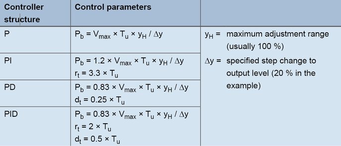
Formulas for setting according to the rate of rise
For a PID controller, the values are obtained with the formulas as follows:

Equation 27

Equation 28

Equation 29
Empirical method for determining the control parameters
With this method, favorable settings for the components P, D and I are determined one after the other. Starting from the original state (output level 0 %), the typical setpoint is always specified; therefore, the method can only be used for relatively fast controlled systems (e.g. fast temperature controlled systems and controlled variables such as speed or flow rate).
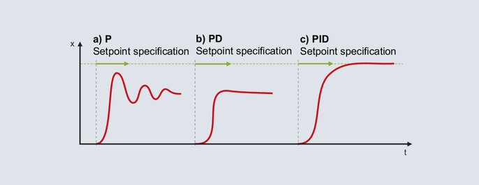
Setting of a PID controller according to the empirical method
The P structure is activated for the digital controller. The proportional band is set relatively large (the dimensioning depends on the controlled system) and the setpoint is specified in the later operating range. The actual value will run sluggishly to the final value and a relatively large control deviation will result. Subsequently, the setpoint is specified with an ever decreasing proportional band XP. The target is an Xp at which the actual value reaches its stable final value after two to three full oscillations (Figure 56a). For a damped start-up, the structure is switched from P to PD. Starting with a small setting for the derivative time, the setpoint is specified with ever increasing Tv. If the process value reaches its final value with the smallest possible oscillation, a favorable Tv is present (Figure 56b).
Note: As soon as the controller sets the output level to 0 % even once during start-up, the Tv is set too high.
With the changeover to PID structure, the I component is activated. The reset time Tn is usually set favorably with four times the value of the previously determined Tv. Figure 56c shows the behavior for a setting Tn = 4 × Tv.
For some lines, not all components can be activated. If a P-structure results in an unsteady behavior already for large settings of XP, neither P- nor D-structure can be used. The I-controller is used.
If the optimization of the P controller was successful, but the introduction of the D component makes the control loop unstable, the PI structure is used.
The application of the presented optimization methods will most likely result in a stable, but not optimal control behavior. Manual post-tuning will further improve the control result. If the behavior of a PID controller can be assigned to one of the curves 62b to 62e, you will find instructions for further optimization below.
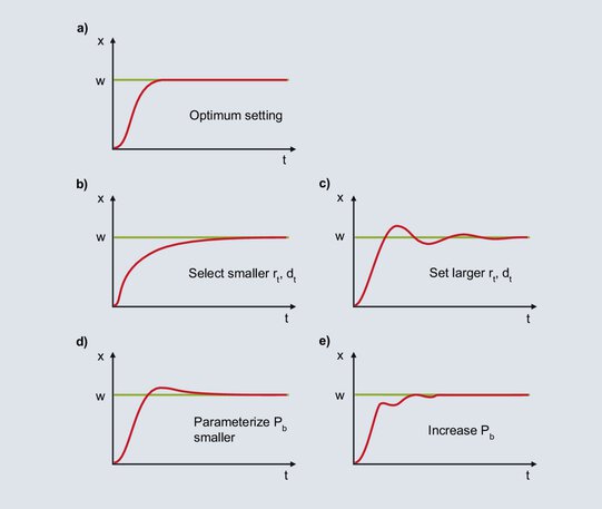
Fig. 62: Notes on the post-tuning of a PID controller
The diagram shows an optimal behavior for a PID controller.
After the setpoint has been specified, the process value increases steeply until the proportional band is reached. When the process value reaches the proportional band, the P component is reduced and the I component ensures that the setpoint value is reached. Due to the relatively large setting of Tn, the increase of the I component is slow and the control deviation is slowly eliminated. For faster integration, Tn must be set smaller; Tv is also reduced according to the ratio Tv/Tn = 1/4.
When the process value enters the proportional band, the I component increases the output ratio. The increase continues until the process value reaches the setpoint. In the case shown, the I component builds up too much output until the control deviation is eliminated, and the process value exceeds the setpoint. With the presence of a negative system deviation, the output level is reduced too quickly, the actual value falls below the setpoint, etc. The symmetrical oscillation of the actual value around the setpoint indicates that Tn is set too small. Tn must be increased and Tv must also be increased according to the ratio Tv / Tn = 1/4.
The I component is formed from the time the process value enters the proportional band until the control deviation is eliminated. Due to the large setting of Xp, the I component starts to form the output ratio already at a large control deviation. Due to the large control deviation at the beginning, the I component forms its output ratio relatively quickly. When the control deviation is eliminated, the I component is too large and the actual value exceeds the setpoint. With a smaller setting for Xp, the I component starts to build up its output level correspondingly slower only with smaller control deviations. The one-time overshoot shown becomes less likely.
If XP is set too low, the output level of the P component is reduced shortly before the setpoint is reached. When the process value enters the proportional band, the P component is reduced very much and the process value drops. Due to the larger control deviation, the output ratio increases and the actual value rises. In the proportional band, small changes in the actual value lead to large changes in the output ratio, which results in a high tendency to oscillation. Calming down is achieved by increasing the proportional band.